Calibrating LLM classification confidences

Introduction

Classification is a common machine learning task. As the field has developed, we have gone from requiring 10,000s of labeled samples per class to just a handful. And with the introduction of Generally Trained Large Language Models (LLMs), we can now classify text content with strong zero-shot accuracy. This means you can provide a text input to the model and it will classify it out-of-the-box, without you having to train it with an annotated dataset.

However, in many practical applications, it is not enough to just classify the text. We also want to know how confident the model is in its decision. For example in a content moderation workflow, one might want to flag low-confidence predictions for human review, while letting high-confidence predictions automatically pass through. If confidence scores are wrong, this workflow breaks down.

In this post, we analyze confidence estimates of OpenAI’s most recent flagship model, GPT-4o, and see how they change with calibration. We do this using two methods. In the first, GPT Self, we ask the LLM to provide a confidence score along with the predictions, resulting in a “self-assessed” confidences. In the second, GPT Logprob, we read out the log probabilities returned by the OpenAI API.

Calibration is a technical term that refers to the agreement between the predicted confidence of a model and the true accuracy of the model. For example, if a model predicts a confidence of 0.8, we would expect that 80% of the samples with that confidence are correct. The sci-kit learn library has a good write-up on the topic.

Related work

There is a large body of work on the general problem of calibrating confidence estimates from machine learning models. For example Geo et al. look at several post-hoc calibration methods in their paper On Calibration of Modern Neural Networks and find that a simple one-parameter calibration method often works well. They also look at how neural networks of different sizes and architectures are calibrated and conclude that larger networks tend to be worse calibrated.

In order to use such post-hoc calibration methods with LLMs, one needs to aggregate the log probabilities of the output tokens. For example, one might average the log probability over the answer, or force the LLM to answer with a single token. Wightman et. al in Strength in Numbers: Estimating Confidence of Large Language Models by Prompt Agreement use a prompt-ensemble method to improve calibration of the log probabilities.

Other methods include the circuitous method of using the LLM to generate examples of each class, extract features from these examples, and then train a classifier on these features. The authors behind the popular Lamini package take this route.

Lin et. al show in Teaching models to express their uncertainty in words that LLMs can be fine-tuned to provide calibrated self-assessed confidences, but they do not investigate self-assessed zero-shot confidence estimates.

In this post we’ll look at post-hoc calibration of self-assessed and log probabilities for zero-shot classification.

Method

Data

We use 12 text classification datasets from our production database. These are real customer use-cases spanning several industries: lead scoring, spam filtering, content moderation, sentiment analysis, topic categorization, and more. Each dataset has between 1,000 and 10,000 annotated samples and between 2 and 10 classes.

Each set is split 20/20/60% into test, calibration, and train. The calibration set is used to calibrate the model, and the test set is used to evaluate the calibration error. Since the LLM is zero-shot, the train set is used only for the transfer learning baseline (more on this later). The test and calibration sets are between 100 and 1000 samples each.

GPT self-assessed

We use the Chat Completion API from OpenAI with the following template.

response = self._client.chat.completions.create(
      model=self._model_name,
      messages=[{"role": "system", "content": prompt}, {"role": "user", "content": content}],
      temperature=0.7,
      max_tokens=4096,
      top_p=1,
  )

Here content is the text content to be classified, and prompt is the prompt to the model. We use the following prompt template:

You will be provided with a {text_type}, and your task is to classify it into categories: {label_list}. 
You should also provide a confidence score between 0 and 1 to indicate how sure you are in the categorization.
End your reply with a json-formatted string: {"label_name": "category", "confidence": <float>}

text_type can be, for example, “news article”, “tweet”, “customer feedback”, etc. label_list is the list of classes in the dataset.

The LLM reply is then parsed from a JSON body and the predicted class and confidence are retrieved.

GPT Log Probabilities

For this, we use the same Chat Completion API, but set logprobs=True. This returns the log probabilities of each token in the API response.

When interpreting the replies, one has to be aware that the same reply can be composed in multiple ways. For example, the label “IceHockey” can be composed by tokens “I” + “ce” + “Hockey” or “Ice” + “Hockey”. So, the LLM would “reserve” some probability mass for both options, even though they amount to the same label. To avoid this, we ask the LLM to reply only with a single character. An example prompt would look as follows:

"You will be provided with an animal sound, and your task is to classify it into categories: dog, cat.

Reply only with a single character according to this mapping: {'a': 'dog', 'b': 'cat'}"

The result is then mapped back to the label and the log probability read from the API response.

Transfer learning baseline

We use a transfer learning baseline. A Logistic Regression (LR) classifier is trained on BERT features extracted from the text content. This is a strong baseline: Logistic Regression is well calibrated in the binary case. Note that this classifier is not zero-shot – it requires labeled training data.

Calibration

Calibrating a classifier is the process of adjusting the predicted confidence of the classifier to better reflect the true accuracy of the model. It’s a common technique, and the basic method is straightforward.

• Predict class and confidence on a hold-out (annotated) calibration set.
• Bucket the predictions by confidence, say in 10 buckets.
• For each bucket, calculate the true accuracy of the model.
• Fit a calibration model to “correct for” the discrepancy between the predicted confidence and the empirical accuracy.

So, for example, if we see that the model is overconfident in the 0.8-0.9 bucket, we can adjust the probabilities in that bucket to better reflect the empirical accuracy.

We use the CalibratedClassifierCV class from Scikit learn to do the calibration, using the default parameters. This method requires a classifier that has a predict_proba method, which the LLM does not have in of itself. To achieve this we take the predicted confidence and convert it to the expected output format: [p1, p2, …, pN], where p1 is the probability of class 1, p2 is the probability of class 2, etc. We set the confidence of the predicted class to the predicted confidence, and the confidence of each of the other classes to (1 - predicted confidence) / (class count - 1). For example, if the LLM gives an 80% confidence for the second class of a three-class problem, we’d build a probability vector like so: [0.1, 0.8, 0.1].

Scoring

We use the Expected Calibration Error (ECE) introduced by Naeini et. al in Obtaining Well Calibrated Probabilities Using Bayesian Binning to evaluate the calibration. The ECE is the average difference between the predicted confidence and the true accuracy of the model, weighted by the number of samples in each bucket. The ECE is a number between 0 and 1, where 0 is perfect calibration and 1 is the worst possible calibration.

Results

Accuracy

Let’s start by looking at the accuracy of the three methods.

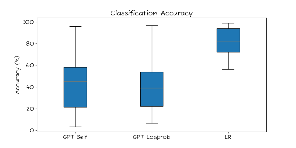
The two LLM methods achieve similar accuracy, while the transfer learning baseline is quite a bit stronger (but this is expected as it is trained on labeled data). More on accuracy in this post.

Confidence estimates

Let’s look at the raw confidence estimates.

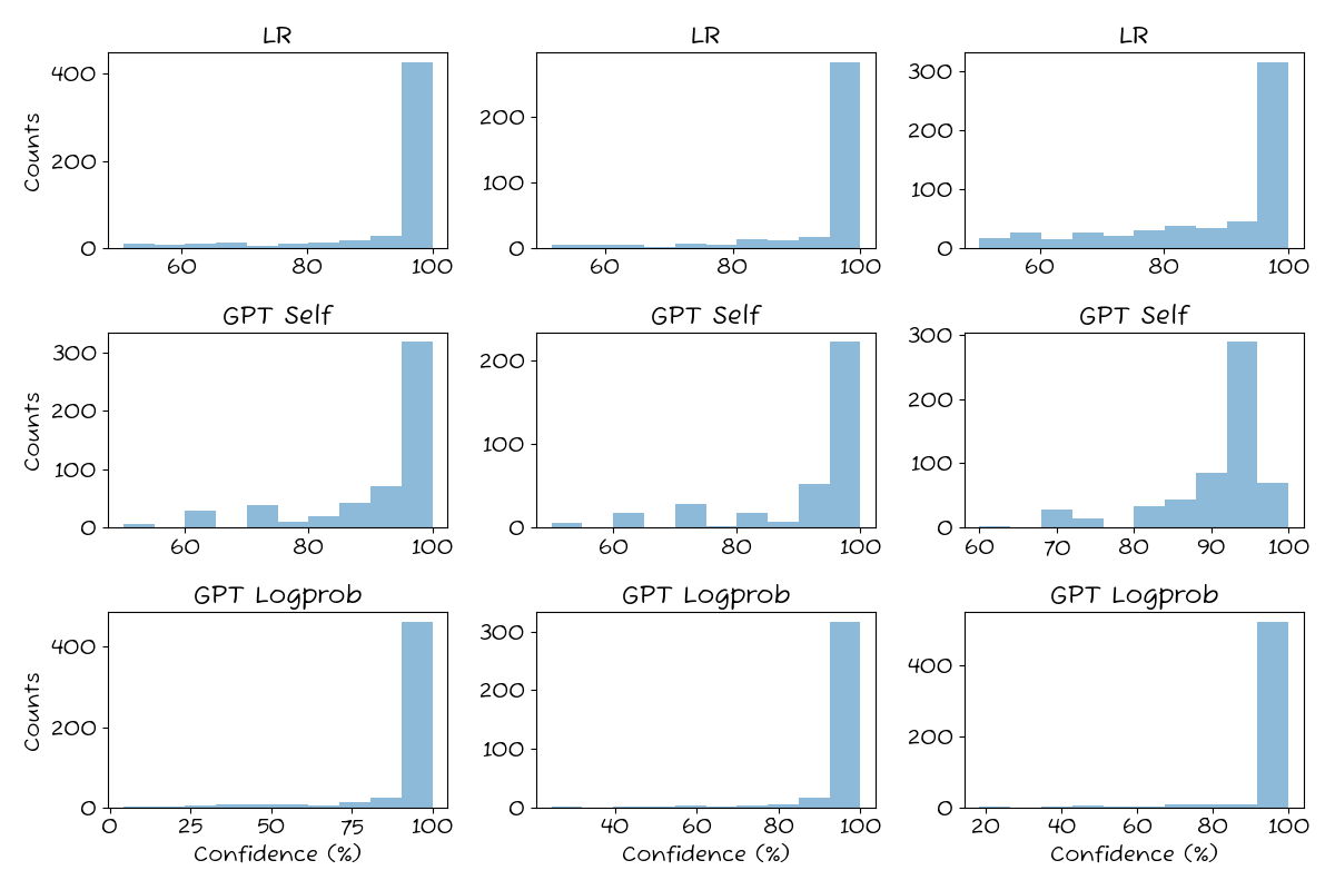
All three methods follow the same general pattern with a high density of high-probability (>90%) predictions. It’s most extreme for GPT Logprob, which almost exclusively returns very high confidences. GPT Self has the most low-confidence predictions, but it exhibits a curious behavior where it tends to return specific confidence estimates over and over, resulting in “missing” values.

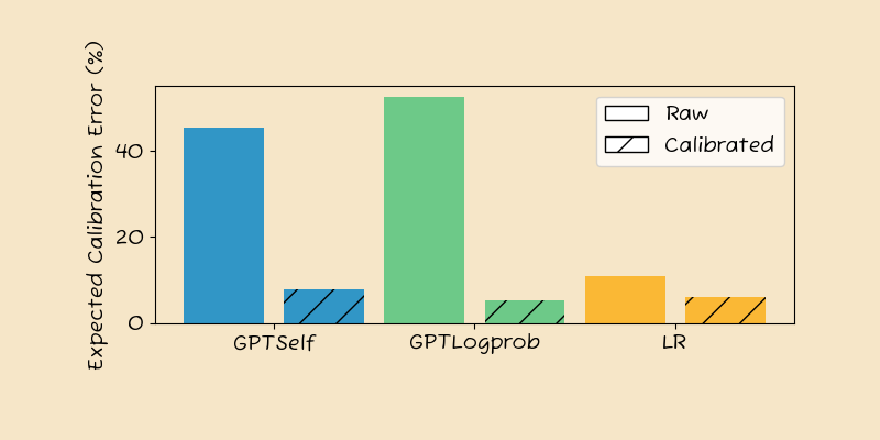
Confidence Calibration

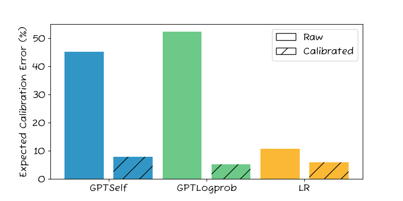
Looking at the main results aggregated across the 12 data-sets, we see that the raw confidence estimates from the GPT methods are not well calibrated. The calibration error is around 45%, which is very high – 4x that of Logistic Regression baseline (11%). GPT Logprob shows an even worse calibration error, at almost 50%.

Fortunately, calibration brings all methods down to below 10%, with GPT Logprob the best at 5%, followed by LR (6%) and GPT Self (8%).

Let’s look at some details next.

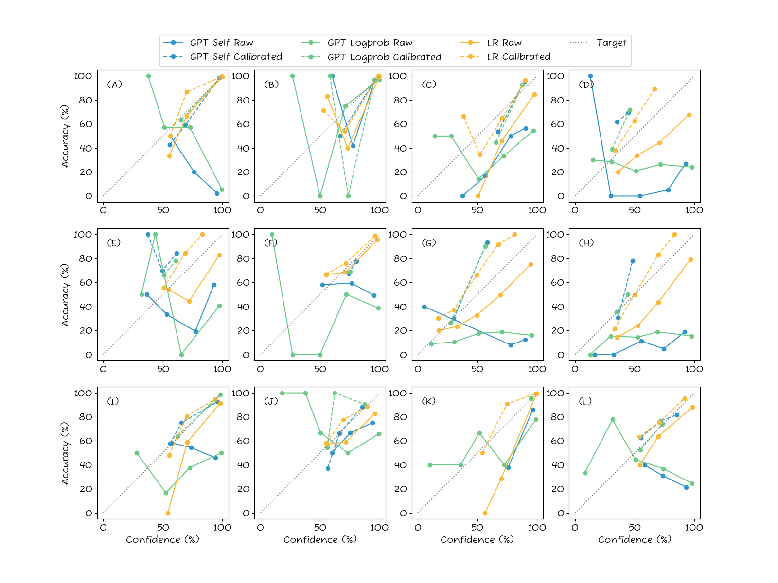
Consider subplot (A) to understand what we are looking at. First, we note that the Raw LR predictions are well calibrated as they tend to follow the diagonal. After calibration, the LR predictions are slightly worse, which seems odd. However, this is not an issue with the method; rather, the reason is simply that both the calibration procedure and the test sets are of limited size (a few 100 samples), and so the calibration parameters are either slightly miscalculated due to the small calibration set, or the evaluation is not “fair” due to small test set.

For both GPT methods, the raw predictions are not well calibrated. Indeed, there is an inverse correlation between how confident the model claims to be and how accurate it is. After calibration, though, the lines look much better.

Now, to the results.

The detailed results underscore the main finding: the self-assessed GPT classification confidences are problematic. In subplots (A), (F), and (L), there is an inverse correlation between confidence and accuracy. The more confidence the LLM claims to be, the more likely it is to make a mistake! In others like (D) and (H), there is no correlation at all between accuracy and confidence.

After calibration, though, the LLM confidences are much better, such as in subplot (A). However, after calibration there is the undesirable effect of score “collapse”. Consider, for instance, at subplots (D) where the calibrated GPT confidences have collapsed into a very narrow band between 0.5. So, while the confidences are now well-calibrated, they are not informative. This is also the case in (F), (H), and (K). This collapse is a consequence of flat accuracy plots. Look at GPT Logprob in plot (D) for example. The initial line shows the same accuracy of around 30% regardless of confidence estimate. So, the best the calibration method can do is to always say 30% confidence. The confidences are now correct, but collapsed and uninformative.

The baseline behaves largely as expected. The raw LR predictions are well-calibrated, except for any dataset with more than two classes. In these cases, LR tends to underestimate the confidence, which is a known issue. The calibration step fixes this and gives a generally well-calibrated confidence estimate.

Conclusion

Using LLMs like ChatGPT to classify data is a convenient way to get off the ground quickly.

However, should your application require accurate confidence estimates, be aware that the confidences are not well-calibrated. In some datasets, a higher confidence actually indicates a larger risk of misclassification!

As shown in this post, the LLM confidences can indeed be calibrated to correctly reflect the expected accuracy, although the resulting scores may suffer from “collapse” and not be very informative.

And since calibration requires annotated data anyway, at that point you may be better off using transfer learning vs an LLM, as this tends to give higher accuracy and more predictable confidence estimates.